You are here
Enter the matrices!
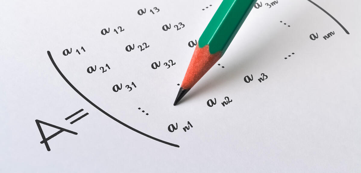
Excel spreadsheets, climate modelling, simulating the structure of an airplane wing, neural network calculation, image processing…Often hiding behind these objects or problems are matrices. Directly derived from algebra, they are mathematical objects on which – as is done with numbers – operations can be performed. These include multiplication which, albeit simple, can require enormous computational resources when the matrix in question is large. That is why researchers have been striving since the 1960s to identify optimised multiplication methods, with a view to accelerating these calculations.
Matrices can be seen as a table of values. Among other things, they make it possible to compactly describe a system of linear equations. Most physical, chemical, and biological phenomena can be represented in the form of matrices. The latter can also be used to characterise an object – such as an image described by a table indicating the value (colour, position, etc.) of each of its pixels – as well as in machine learning, where “most of the calculation in neural networks is conducted on matrices representing the state of each of these neurons”, points out Gabriel Peyré, a researcher in the Department of Mathematics and Applications at the École Normale Supérieure1.
From tables to matrices
The ancestor of the matrix was born in China circa the 1st century BC or AD. “In the anonymous work The Nine Chapters on the Mathematical Art, there is something resembling a matrix. The procedure for solving a linear system actually began by describing the arrangement of data in a table,” explains Karine Chemla, a researcher in the history of mathematics at the SPHERE laboratory2. The interest of this layout is similar to our positional numbering, which facilitates addition by superimposing units, tens, hundreds, etc. “The idea is that the algorithm for solving the problem is based on arranging data in a table.”
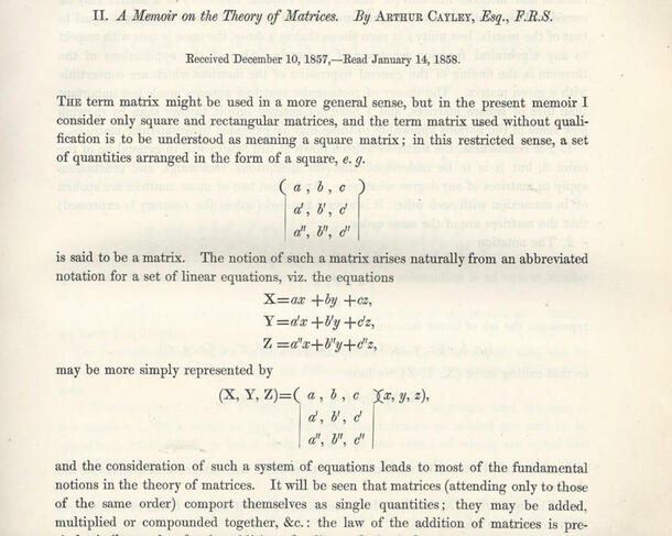
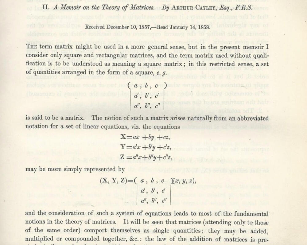
However, these tables could not be considered matrices, for they cannot be used to conduct operations. “This leap forward would come in the mid-nineteenth century with the work of Arthur Cayley.” This British mathematician performed the first elementary operations using these objects, namely addition, inversion, and multiplication. Doing so on these matrices allowed him to solve geometry problems, since these can write out the geometric transformation of an object, such as its rotation. The succession of multiple transformations is quite simply the multiplication of matrices, each representing a geometric transformation that the said object would undergo. This technique is widely used in 3D graphics.
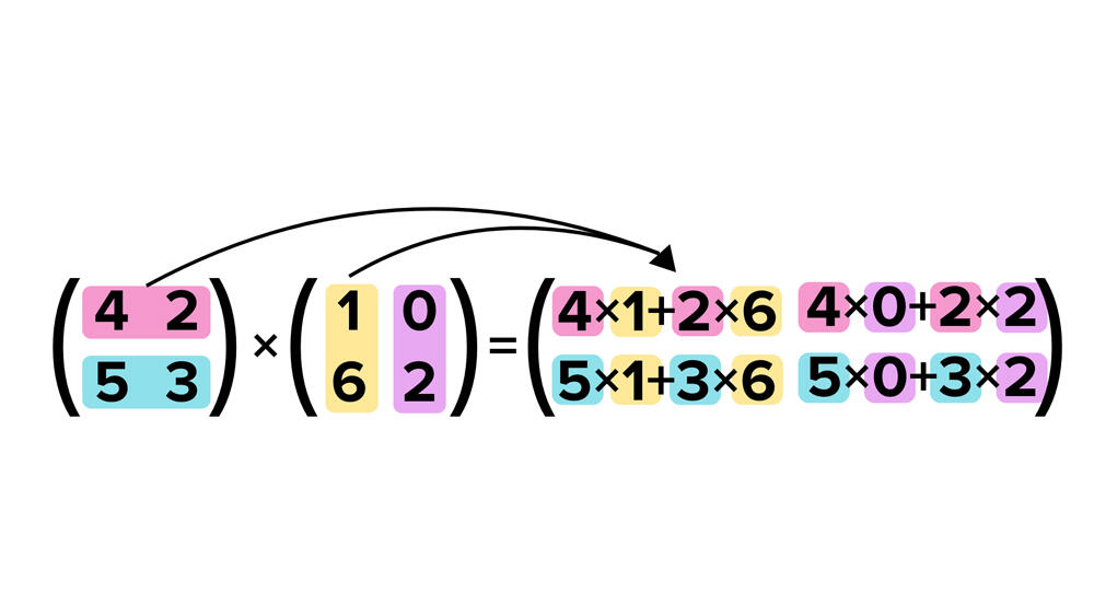
In an ever more digital world, matrix multiplication has become central, and not just in mathematics. “Almost all algorithms use matrix multiplication for numerical solution,” reminds François Le Gall, a researcher at the Graduate School of Mathematics at Nagoya University (Japan). The advantage is that the trivial (or standard) method for conducting this operation is simple to perform by hand or with a computer, as long as the matrix is of reasonable size. The disadvantage is that the number of computational steps needed for this algorithm increases exponentially with matrix size. “We can count the additions and multiplications needed to multiply two matrices with the trivial algorithm. For a matrix with n rows and n columns, this cost, which is known as ‘algorithm complexity,’ is n3,” explains Clément Pernet, an academic at the Jean Kuntzmann laboratory3. For instance, if two matrices have 1,000 rows and 1,000 columns each, then the computer (or human) must perform 1 billion operations (or 1,0003) to successfully multiply them. “As it happens, matrices of such size are in fact common in applications, especially in machine learning,” stresses Le Gall.
A quest for the best algorithm
In the 1960s, mathematicians and computer scientists wondered whether matrices could be multiplied with fewer operations. “Volker Strassen was convinced it was not possible. It was nevertheless he who discovered an algorithm that can solve a matrix product in less than n3 steps,” says Pernet with a wry smile. This discovery launched a quest for the optimal algorithm for matrix products! “The primary motivation is to conduct calculations quickly,” adds Le Gall. Indeed, multiplying two matrices takes time: 30 seconds for two matrices of 10,000 rows and 10,000 columns, but 4 minutes with twice the number of rows and columns. Finding an algorithm that reduces the number of calculation steps would reduce overall computation time. This reduction is all the more discernible as matrix size increases.

Let us compare the trivial algorithm to a hypothetical multiplication algorithm whose complexity is n². During the multiplication of the two matrices measuring 3x3 in size, the advantage of the second method over the trivial algorithm is not that significant. However, if the size of the matrix is a million rows and a million lines, the second algorithm would require a million fewer calculations, or a million times less time and energy. “Our theoretical motivation is also to understand how far we can reduce the value of the power of n,” adds Le Gall. What we know is that even when optimised, the algorithm cannot go below a complexity of n2, which is the number of cells in the result matrix, hence a minimum of n2 steps are needed to write out the result. To reduce complexity, researchers are concentrating their efforts on lowering the number of multiplications required before solving a matrix product. “We know the number of additions that must be carried out, and it is small in relation to the number of multiplications. So it is the latter in particular that determine the power of n.”
A hardly lesser complexity
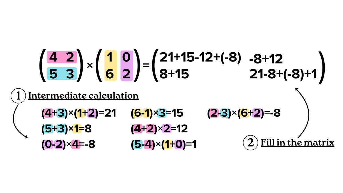
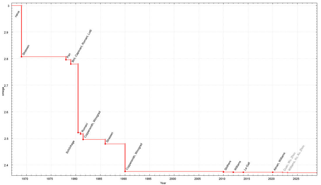
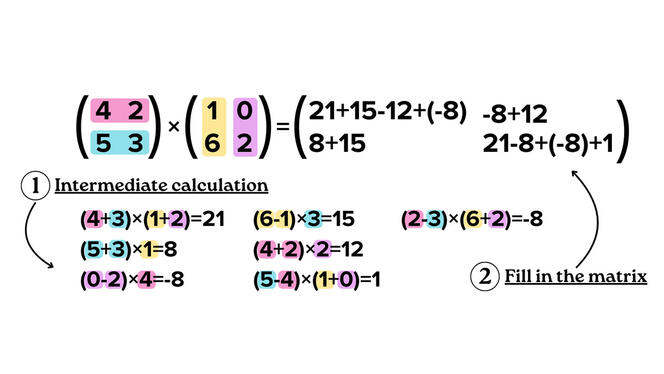
The first improvement, Volker Strassen’s algorithm, reduced the complexity of n3 to n2.807. He used the divide-and-conquer method, consisting in decomposing the problem (here the matrix) into multiple sub-problems (parts of the matrix), and those in turn into other sub-problems, until arriving exclusively at matrices measuring 2 x 2 in size. All that remains is to multiply these results to arrive at the final solution. In this way the multiplication of two matrices measuring 2 x 2 in size requires one less multiplication than the trivial method, and the multiplication of matrices measuring 10,000 x 10,000 offers a time savings of approximately 28%. “After Volker Strassen, there was no progress for ten years. Then, between 1978 and the late 1980s, competition was fierce!" A number of small improvements were discovered, initially thanks to the ongoing research of Strassen, and later to that of the mathematicians Shmuel Winograd and Don Coppersmith, who used another method for decomposing matrices to decrease the complexity to n2.376.
Since the 2010s, advances have successively been made by improving this highly precise method. The final optimisation to date was made by Zhou Renfei and his colleagues at the Institute for Interdisciplinary Information Sciences (IIIS) at Tsinghua University (China) in late 2023, reducing the exponent from 2.372860 to 2.371866. This result may not seem like a great deal, but it is decisive mathematically. “They found that something in the Coppersmith and Winograd method was not optimal. Something we had missed,” congratulates Le Gall.

Along the way, the theoretical motivation has overtaken real improvements. “After the 1970s, matrix multiplication algorithms became galactic,” warns Pernet. In other words, these algorithms are now so complex that they reduce the computation time only for matrices that are so gigantic that all of the computers on Earth would not be enough to store them. In practice, they are never used to multiply two matrices, even those with thousands of rows and columns. However, just because the result is not used does not mean that it is not of interest. “This research provides answers to fundamental questions, and calls for implementing new techniques,” Peyré concludes. This race among theorists could indeed result in algorithms that are both faster and usable in concrete applications.♦


